home..

Pixar’s Box Office Formula: Do Great Stories Make Great Sequels?

March 2025 (2132 Words, 12 Minutes)

“Sequels are not part of our business model. When we have a great story, we’ll do a sequel.” Ed Catmull (Pixar co-founder)

Introduction

“Pixar has stated that, “sequels are not part of our business model.” But what patterns emerge from box office performance and critical reception? As I was learning R, I explored this question using regression modeling.

To immerse myself in real-world data analysis, I joined the Data Science Learning Community on Slack and discovered the #chat-tidytuesday channel. It just so happened to be Tuesday, and a Zoom session was starting in 10 minutes! I listened in as the group explored data from the Long Beach Animal Shelter, and I was fascinated by the many different ways people interpreted the information. Inspired, I decided to join the next TidyTuesday challenge.

In this post, I’ll walk through how I analyzed Pixar Data, from obtaining and tidying the data to visualizing the results. If you’re new to R and enjoy working with real-world datasets, you’ll find this especially useful!

The Goal

The aim of this project was to fit a regression model to the Pixar dataset, focusing on understanding interaction effects between variables and visualizing the results in a meaningful way.

While the data manipulation itself is relatively straightforward, this project serves as an exercise in applying key concepts from Chapter 3: Linear Regression. As I continue learning R and working with linear models, I saw this week’s TidyTuesday dataset as an opportunity to reinforce my understanding through hands-on analysis.

For this analysis, I used the {pixarfilms} R package by Eric Leung, available through the TidyTuesday GitHub repository.

The {pixarfilms} package provides datasets to explore Pixar films, including details on production, box office performance, and reception. Most of the data is sourced from Wikipedia.

My approach involved:

Data extraction – Loading the dataset from {pixarfilms}
Data cleaning – Transforming the data for analysis
Modeling – Fitting a linear regression model and examining interactions
Visualization – Creating meaningful plots to interpret findings

Getting Started

First, I loaded the necessary packages in R:

library(dplyr)
library(readr)
library(lubridate)
library(pixarfilms)
library(ggplot2)
library(scales)
library(tidyr)
library(stringr)
theme_set(theme_light())

Obtaining the Data

The dataset comes from two sources:

The TidyTuesday Pixar dataset (March 11, 2025), which provides information on Pixar films, including box office revenue, production budgets, and audience reception.
The {pixarfilms} R package by Eric Leung, which contains additional financial data on Pixar films.

I imported the data using readr::read_csv() for the TidyTuesday dataset and loaded the {pixarfilms} package for additional box office data:

# Read the TidyTuesday datasets
pixar_films_raw <- readr::read_csv('https://raw.githubusercontent.com/rfordatascience/tidytuesday/main/data/2025/2025-03-11/pixar_films.csv')

public_response_raw <- readr::read_csv('https://raw.githubusercontent.com/rfordatascience/tidytuesday/main/data/2025/2025-03-11/public_response.csv')

# Load box office data from pixarfilms package
box_office_raw <- pixarfilms::box_office

Let’s start by examining the data. I used View() and the standard head() function to take a quick look at the dataset. Below is a preview of the first few rows of pixar_films_raw:

# A tibble: 6 × 5
   number film           release_date run_time
   <dbl> <chr>          <date>       <dbl>  
1       "Toy Story"      1995-11-22      81  
2       "A Bug's Life"   1998-11-25      95  
3       "Toy Story 2"    1999-11-24      92  
4       "Monsters, Inc." 2001-11-02      92  
5       "Finding Nemo"   2003-05-30     100  
6       "The Incredibles" 2004-11-05    115  

Data Cleaning and Identifying Sequels

First, I created a new column to indicate whether a film was a sequel. Since the dataset doesn’t explicitly label sequels, I manually identified them using a list of known Pixar sequels.:

# Define a vector of known sequels
sequel_titles <- c("Toy Story 2", "Toy Story 3", "Toy Story 4",
                   "Cars 2", "Cars 3", "Finding Dory", 
                   "Incredibles 2", "Monsters University", "Lightyear")

# Create the is_sequel column
pixar_films <- pixar_films_raw %>%
  select(-number) %>%
  mutate(is_sequel = ifelse(film %in% sequel_titles, 1, 0))

In the pixar_films dataframe I picked off the first column, “number” that just contained a bunch of numbers using select(). This new is_sequel column allows us to compare sequels and original films in later analyses.

Converting Review Scores

The public_response dataset includes various critic and audience ratings, such as Rotten Tomatoes scores, Metacritic scores, and CinemaScore letter grades. Since CinemaScore ratings are given as letters (e.g., “A+”, “B-“), I converted them into a numeric scale for easier comparison:

# Define a conversion table for CinemaScore grades
score_conversion <- c("A+" = 100, "A" = 95, "A-" = 90, 
                      "B+" = 85, "B" = 80, "B-" = 75, 
                      "C+" = 70, "C" = 65, "C-" = 60, 
                      "D+" = 55, "D" = 50, "D-" = 45, 
                      "F" = 0)

# Convert letter grades to numeric scores and handle missing values
public_response <- public_response_raw %>%
  mutate(cinema_score = score_conversion[cinema_score]) %>%
  mutate(across(c(rotten_tomatoes, metacritic, cinema_score, critics_choice), ~replace_na(.x, 0)))

By converting these letter grades, I ensured they could be used in statistical models without issues. With these transformations complete, I was ready to visualize how critics’ ratings compared across Pixar films

Creating the Heatmap

With the data in the right format, I used ggplot2 to generate a heatmap. Each tile represents a Pixar movie’s rating from a specific critic, with colors indicating the score—red for lower ratings and green for higher ratings.

# Heatmap for critics score
ggplot(critics_long, aes(x = critic, y = film, fill = score)) +
  geom_tile(color = "white") +
  scale_fill_gradient(low = "red", high = "green") +
  labs(title = "Pixar Movie Critic Score Heatmap",
       x = "Critic", y = "Movie", fill = "Score")

Final Visualization

Here is the resulting heatmap! Pixar Movie Critic Score Heatmap

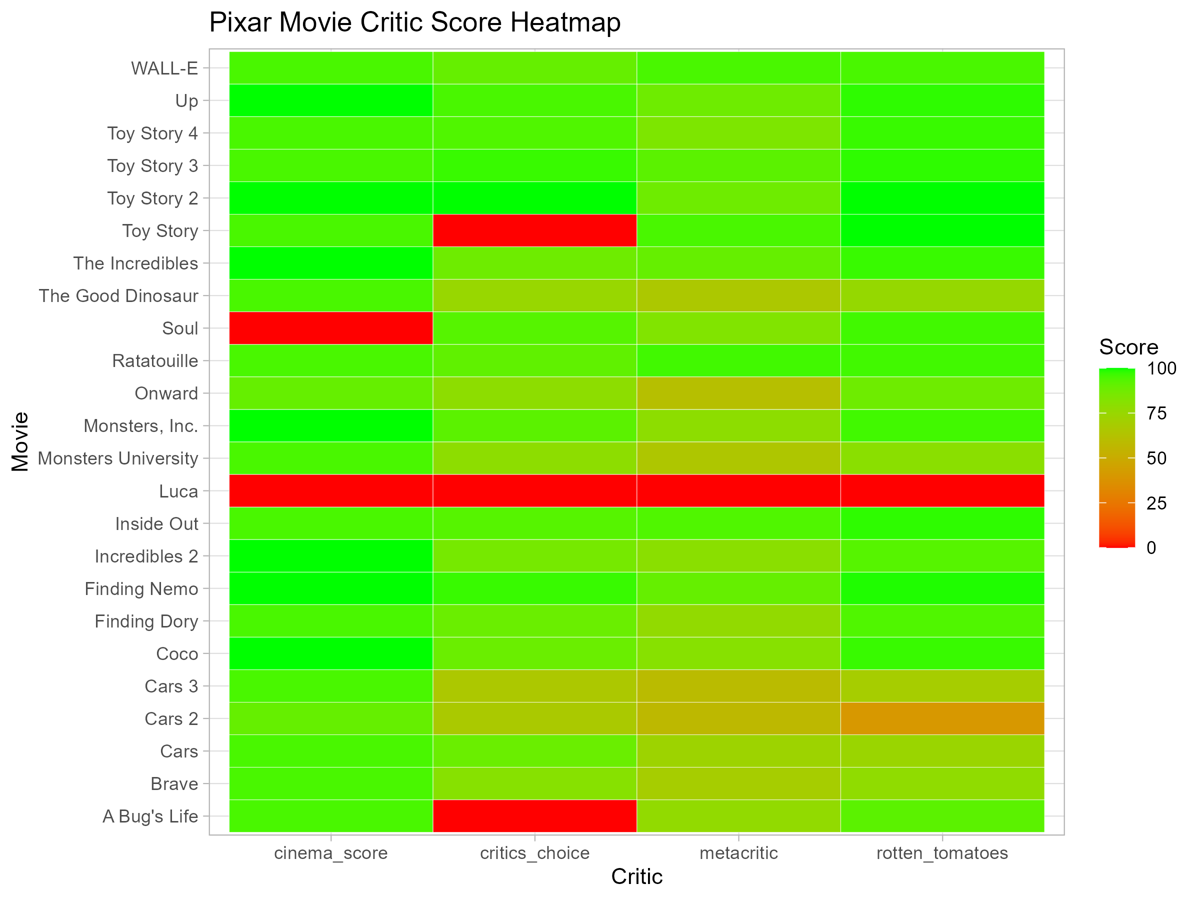
Looking at this, I noticed that CinemaScore ratings didn’t vary much, while Metacritic scores showed a wider range of opinions. Another interesting detail—Luca is missing data. I kept it in the visualization because it’s best practice not to remove missing values without considering their context.

Do Box Office & Reviews Predict Pixar Sequels?

To explore this, I built a logistic regression model, examining how factors like Metacritic score, box office revenue in the U.S. and Canada, and budget are associated with the likelihood of a Pixar movie being a sequel.

Metacritic score (critical reception)
Box office revenue in the U.S. and Canada (financial success)
Budget (how much Pixar invested in the first film)

Since our outcome variable (sequel or not) is binary (1 or 0), a logistic regression model is the best fit. Unlike linear regression, which predicts continuous values, logistic regression estimates probabilities—allowing us to understand what factors increase the odds of a sequel being made.

Here’s the R code:

sequel_model <- glm(is_sequel ~ metacritic + box_office_us_canada + budget, 
                    data = box_office_data, family = binomial)
summary(sequel_model)

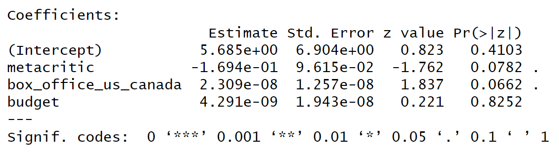
Resulting in: Logistic Linear Model Comparing if a Sequel is Made to coefficients

The coefficients tell us how much each factor influences the odds of a sequel. A positive coefficient means the variable increases the likelihood of a sequel, while a negative coefficient decreases it.

Visualizing Sequel Probabilities

To better understand these patterns, I plotted the predicted probability of a sequel against box office earnings in the U.S. and Canada.

Generating the Plot

I first used the predict() function to compute sequel probabilities from the regression model:

# Generate predicted probabilities
box_office_data <- box_office_data %>%
  mutate(predicted_sequel_prob = predict(sequel_model, type = "response"))

Create the plot

# Create the plot
ggplot(box_office_data, aes(x = box_office_us_canada, y = predicted_sequel_prob)) +
  geom_point(aes(color = as.factor(is_sequel)), size = 3) +
  geom_smooth(method = "glm", method.args = list(family = "binomial"), se = FALSE) +
  scale_x_continuous(labels = scales::dollar_format()) +  # Format x-axis as dollars
  labs(
    title = "Predicted Probability of a Pixar Sequel",
    x = "Box Office Revenue (US & Canada)",
    y = "Predicted Sequel Probability",
    color = "Sequel"
  )

Final Visualization

Here’s the resulting plot:

Pixar Sequel Probability Plot

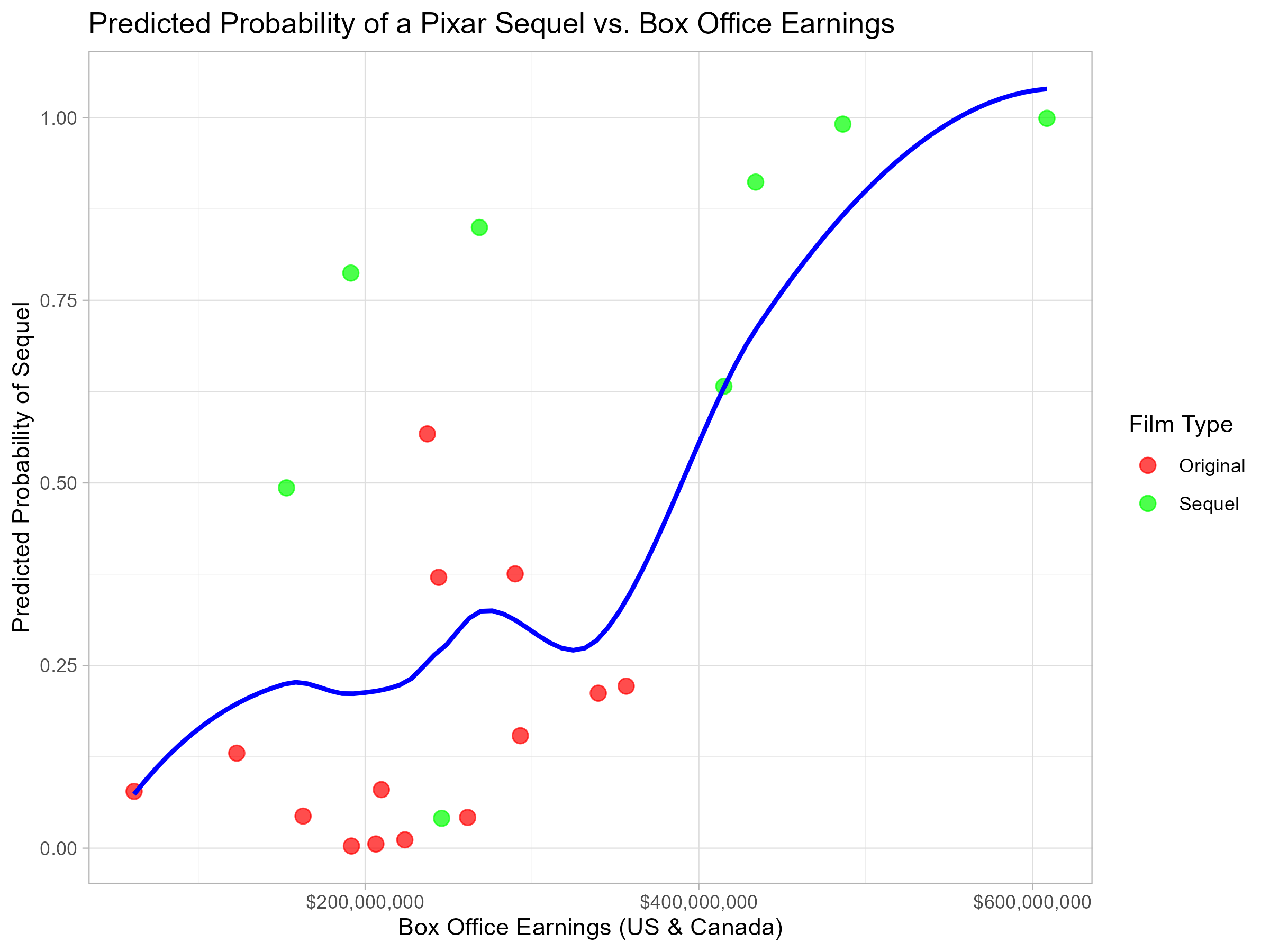
Each point is a Pixar film. The blue curve shows how higher box office earnings increase the probability of a sequel.

Looking at the trend, we can see that higher box office earnings tend to increase the probability of a sequel. This supports our earlier finding that financial success is a key factor in Pixar’s sequel decisions.

Interpreting the Results

So what patterns did the data reveal?

🎬 Box Office Revenue Matters! (p = 0.0662) → This is the strongest predictor. More money at the box office = higher odds of a sequel.
🤔 Do Critics Matter? (p = 0.0782) → Weak evidence suggests that movies with lower Metacritic scores might be more likely to get sequels (which is surprising!).
💰 Budget? Not Important. (p = 0.8252) → Pixar’s initial investment in a film doesn’t seem to impact whether they greenlight a sequel.

While none of these predictors meet the strict p < 0.05 threshold, box office revenue has the strongest relationship, suggesting that financial success may be a consideration in Pixar’s sequel decisions.

So, despite Ed Catmull’s statement, money does seem to play a role in Pixar’s sequel decisions. 🎬💰

Key Takeaways

1. Box office success is associated with sequels – Movies that perform well financially tend to have a higher probability of getting a sequel.

2. Critical reception shows a weaker effect – There is some evidence suggesting that lower Metacritic scores might be linked to sequel production, but it’s not conclusive.

3. Budget doesn’t appear to be a strong factor – The initial production budget of a film doesn’t seem to have a significant relationship with whether Pixar greenlights a sequel.

This project reinforced my understanding of data wrangling, visualization, and animation in R. If you’re interested in trying a similar analysis, I highly recommend TidyTuesday as a great place to start!

Let me know what you think!